tidydice

Simulates Dice Rolls and Coin Flips.

Introduction

A basic understanding of probability and statistics is crucial for data understanding. A great way to teach probability and statistics is to start with an experiment, like rolling a dice or flipping a coin.

This package simulates rolling a dice and flipping a coin. Each experiment generates a tibble. Dice rolls and coin flips are simulated using sample(). The properties of the dice can be changed, like the number of sides. A coin flip is simulated using a two sided dice. Experiments can be combined with the pipe-operator.

Installation

CRAN

install.packages("tidydice")

DEV version (github)

# install from github
if (!require(devtools)) install.packages("devtools")
devtools::install_github("rolkra/tidydice")

if you are behind a firewall, you may want to:

• Download and unzip the tidydice package
• Then install it with devtools::install_local

# install local
if (!require(devtools)) install.packages("devtools")
devtools::install_local(path = <path of local package>, force = TRUE)

Basic example

Let’s roll 60 dice:

# load packages
library(tidydice)

# roll 60 dice (10 x 6 dice = 60)
data <- roll_dice(times = 10, rounds = 6)
data

We get tidy data, where each row is a dice. It is a success, if the result is a 6.

# A tibble: 60 × 5
   experiment round    nr result success
        <int> <int> <int>  <int> <lgl>  
 1          1     1     1      5 FALSE  
 2          1     1     2      6 TRUE   
 3          1     1     3      6 TRUE   
 4          1     1     4      1 FALSE  
 5          1     1     5      5 FALSE  
 6          1     1     6      1 FALSE  
 7          1     1     7      4 FALSE  
 8          1     1     8      5 FALSE  
 9          1     1     9      1 FALSE  
10          1     1    10      2 FALSE  
# … with 50 more rows

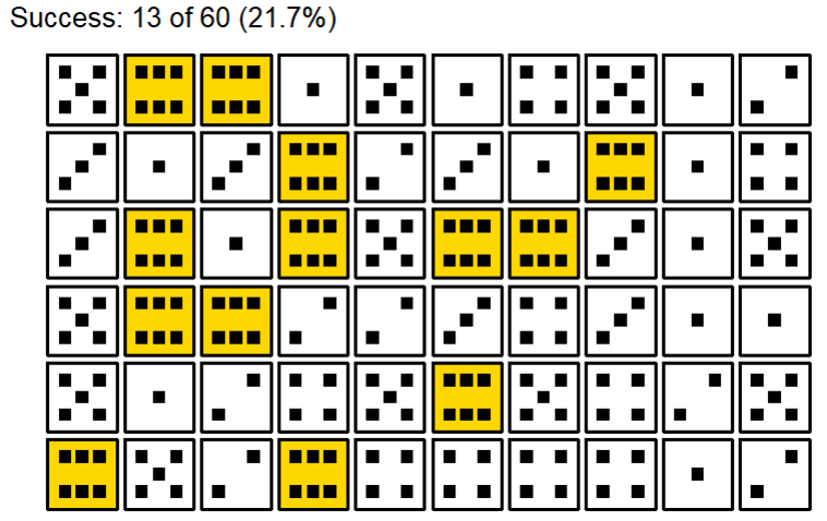
Now let’s plot it:

data |> plot_dice()

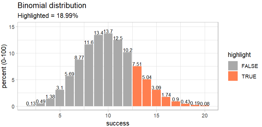
We got 13 six. Is this unlikely? The expected value is 10 (60 dice / 6 sides = 10). So 13 is more than expected, is it a sign of cheating? Let’s check using the binomial ditribution:

# binomial distribution
binom_dice(times = 60) |> 
  plot_binom(highlight = c(13:60))

The binomial distribution shows, that there is a 19% chance that you can get 13 or more six using a fair dice.

Roll dice

# load packages
library(tidydice)

# roll a dice
roll_dice()

# roll a dice 6x
roll_dice(times = 6)

# roll a dice 6x and plot result
roll_dice(times = 6) |> 
  plot_dice()

# repeat 6x
roll_dice(times = 6, rounds = 6)  |>  
  plot_dice()

# count success per round
roll_dice(times = 6, rounds = 6, agg = TRUE)

# Binomial distribution
binom_dice(times = 6)
  
# Binomial distribution + plot
binom_dice(times = 6) |>  
  plot_binom()

# Binomial distribution + plot 
binom_dice(times = 6) |>  
  plot_binom(highlight = 0:2)

Roll dice (advanced)

To do more complex dice rolls use roll_dice_formula():

library(tidydice)

roll_dice_formula(
  dice_formula = "4d6e3", # 4 dice with 6 sides, explode on a 3
  rounds = 5,             # repeat 5 times
  success = 15:24,        # success is defined as sum between 15 and 24
  seed = 123              # random seed to make it reproducible
)

• 1d6 = roll one 6-sided dice
• 1d8 = roll one 8-sided dice
• 1d12 = roll one 12-sided dice
• 2d6 = roll two 6-sided dice
• 1d6e6 = roll one 6-sided dice, explode dice on a 6
• 3d6kh2 = roll three 6-sided dice, keep highest 2 rolls
• 3d6kl2 = roll three 6-sided dice, keep lowest 2 rolls
• 4d6kh3e6 = roll four 6-sided dice, keep highest 3 rolls, but explode on a 6
• 1d20+4 = roll one 20-sided dice, and add 4
• 1d4+1d6 = roll one 4-sided dice and one 6-sided dice, and sum the results

Flip coin

# load packages
library(tidydice)

# flip a coin
flip_coin()

# flip a coin 10x
flip_coin(times = 10)

# flip a coin 10x and plot result
flip_coin(times = 10) |> 
  plot_coin()

# repeat 10x and plot result
flip_coin(times = 10, rounds = 10) |> 
  plot_coin()

# count success per round
flip_coin(times = 10, rounds = 10, agg = TRUE)

# Binomial distribution
binom_coin(times = 10)
  
# Binomial distribution + plot
binom_coin(times = 10) |>  
  plot_binom()

# Binomial distribution + plot 
binom_coin(times = 10) |>  
  plot_binom(highlight = 0:2)