
| GRASS 5.7: Vector networking tutorial |
| Example: shortest path vector networking with d.path |
A module based on the DGLib vector network library is 'd.path' (see screenshot which calculates shortest path on a vector network map. Traveling costs may be either line lengths, or costs saved as attributes in a database table (supported are cost assignments for both arcs and nodes).
We want to use the 'roads' map of the Spearfish demo location (if needed, convert to 5.7 format with 'v.convert'). A simple example is to use the vector length as costs:
d.vect roads
d.path map=roads
echo "select * from roads" | db.select
echo "update roads set travelcost=5 where cat=1" | db.execute
echo "update roads set travelcost=20 where cat=2" | db.execute
echo "update roads set travelcost=40 where cat=3" | db.execute
echo "update roads set travelcost=60 where cat=4" | db.execute
echo "update roads set travelcost=80 where cat=5" | db.execute
echo "select * from roads" | db.select
d.path map=roads afcol=travelcost abcol=travelcost
| Reachability of Schools: v.net.iso |
We need a street map and a map of school locations.
A nice, free vector data set is FRIDA,
the vector map of Osnabrück, a city in northern Germany.
Additionally you can download the
related ASTER
DEM at 30m resolution (ARC ASCII GRID raster format, reprojected to
Gauss-Krüger, 700kb).
After downloading the dataset (SHAPE files) and extracting the
related GRASS location (corrected 1 Oct 2004),
we can start. Enter GRASS 5.7 with that osnabrueck LOCATION and user1 mapset.
Translation aid for the map names:
#line/point layers:
v.in.ogr dsn=/ssi0/ssi/neteler/grassdata/osnabrueck/maps output=strassen layer=strassen
v.in.ogr dsn=/ssi0/ssi/neteler/grassdata/osnabrueck/maps output=poi layer=poi
#area layer:
v.in.ogr dsn=/ssi0/ssi/neteler/grassdata/osnabrueck/maps output=gewaesserflaechen layer=gewaesserflaechen
-> WARNING: 2. centroid found in area 30...etc
-> "WARNING: Area boundaries are not cleaned by this module. Run v.clean on
         imported vector on new map ."
v.clean input=gewaesserflaechen output=gewaesserflaechen_clean tool=rmdupl,bpol
v.category poi out=poi_2f field=2 op=add
#verify:
v.category poi_2f field=1,2 op=print
-> field 1 == field 2
v.extract in=poi_2f out=schools type=point where="poiName='Schule' or poiName='Schulen'"
   #TODO: Fix Usulaschule - SQL regex
v.info schools
-> one dblink
v.category schools field=1,2 op=print
-> 2 fields
d.erase
d.vect strassen
d.vect schools disp=attr attr=poiName bgcolor=white bcolor=black
d.vect schools col=red icon=basic/diamond
v.patch in=strassen,schools out=streets_schools
v.info streets_schools
-> dblinks = 0
d.erase
d.vect streets_schools
d.vect streets_schools type=point col=red
db.connect dr=dbf database='$GISDBASE/$LOCATION_NAME/$MAPSET/dbf/'
db.describe -c strassen
ncols:6
Column 1: cat
Column 2: strShapeID
Column 3: strID
Column 4: strTypID
Column 5: strSpuren
Column 6: strEbene
-> the 'cat' column was added by 'v.in.ogr'
v.db.connect streets_schools dr=dbf data='$GISDBASE/$LOCATION_NAME/$MAPSET/dbf/' \
  table=strassen field=1 key=cat

v.db.connect streets_schools dr=dbf data='$GISDBASE/$LOCATION_NAME/$MAPSET/dbf/' \
  table=schools field=2 key=cat
v.db.connect -p streets_schools
Display the patched map with the linked two tables:
d.erase
d.vect streets_schools
d.vect streets_schools type=point col=red disp=attr attrcol=poiName lfield=2
d.what.vect streets_schools
First we generate the connection map between schools and closest streets:
v.distance -p from=schools to=strassen output=streets_schools_connect upload=dist column=dist

d.erase
d.vect strassen col=grey
d.vect schools col=red
d.vect streets_schools_connect col=blue
Then we merge these line connections into the schools_streets map (we have to snap nodes and break street lines at intersection of the connecting lines):
v.patch in=streets_schools,streets_schools_connect out=schools_net

#note: next will also remove the few bridges in the streets_schools map...
v.clean in=schools_net out=schools_net_clean tool=snap,break thresh=1
g.remove vect=schools_net

#since g.rename doesn't exist:
g.copy vect=schools_net_clean,schools_net
g.remove vect=schools_net_clean

d.erase
d.vect schools_net
Now the map containing schools and streets is prepared for network analysis.
d.vect schools_net
#show all schools with their cats:
d.vect schools_net ty=point icon="basic/circle" size=5 col=blue
d.vect schools_net ty=point disp=cat
#next is very slow due to an unsolved bug in graphlib (therefore cache disabled):
#We check for three schools as we give a ccats range:
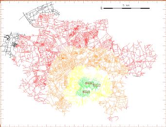
v.net.iso input=schools_net output=schools_iso ccats=200-210 costs=1000,2500,5000,10000
d.erase

#show all streets and schools:
d.vect schools_net

#show reachabilities as calculated above:
d.vect schools_iso col=green  cats=1
d.vect schools_iso col=yellow cats=2
d.vect schools_iso col=orange cats=3
d.vect schools_iso col=red    cats=4

#highlight the selected schools:
d.vect schools disp=attr attr=poiName bcolor=black cat=200-210
d.vect schools_net ty=point cat=200-210 col=red icon="basic/circle" size=5

#nice frame etc:
d.grid -g s=1000
d.barscale -t bc=white tc=black at=60,5
City of Osnabrück - reachability of selected schools (click to
enlarge):

| Creating subnets: v.net.alloc |
TODO better example (below is close to nonsense):
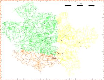
v.net.alloc input=schools_net output=schools_alloc ccats=200-210

#check for present categories (school IDs)
v.category schools_alloc option=print | sort -nu
0
201
204
209

d.erase

#show all streets and schools:
d.vect schools_net

#show reachabilities as calculated above:
d.vect schools_alloc col=green  cats=201
d.vect schools_alloc col=yellow cats=204
d.vect schools_alloc col=orange cats=209

#highlight the selected schools:
d.vect schools disp=attr attr=poiName bcolor=black cat=200-210
d.vect schools_net ty=point cat=200-210 col=red icon="basic/circle" size=5

#nice frame etc:
d.grid -g s=1000lloc col=orange cats=209
d.barscale -t bc=white tc=black at=60,5

| v.net.steiner: optimized connection of nodes on a given vector network |
We use again the City of Osnabrück vector data as above for this fictitious project. First we extract the hospitals from the points of interest map:
v.extract poi out=hospitals where="poiTypID=2"
d.vect hospitals col=green
d.vect strassen
We can see that the hospitals are not yet connected to the streets network, so we have to generate the connecting lines (using the nearest distance search, of course it were more realistic to digitize with 'v.digit' from a street map):
v.distance -p from=hospitals to=strassen output=hospitals_conn_streets upload=dist column=dist
d.vect hospitals col=yellow
d.zoom
d.vect hospitals_conn_streets col=red
d.vect strassen
Patch together the hospital points map, the streets map and the map of connecting lines:
v.patch in=hospitals,hospitals_conn_streets,strassen out=h_network
#note that patch doesn't insert nodes where lines are connecting.
#so we clean it (threshold of 1 millimeter):
v.clean h_network out=h_network_clean tool=snap,break thresh=0.001

#display patched map, with hospital points highlighted:
d.vect h_network_clean
d.vect h_network_clean ty=point col=red
Print the categories for the hospital points:
v.category option=print input=h_network_clean type=point
#the range is from 40-215
Calculate the Steiner tree for broadband cable connection network (slow at time to DGLib cache bug):
v.net.steiner in=h_network_clean output=broadband_map afield=1 nfield=1 nsp=-1 tcats=40-300
Let's study the result:
d.erase
d.vect strassen
d.vect hospitals col=yellow
d.vect broadband_map col=red
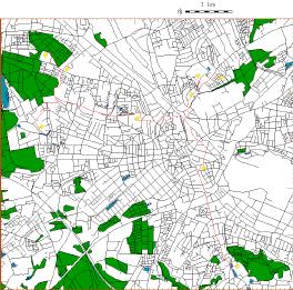
City of Osnabrück - optimal broadband connection of hospitals for
telemedicine applications (click to enlarge):

| v.net.salesman |
Think that you should introduce medical equipment to all hospitals in the town. You want to minimize the travel route. This is the traveling salesman problem, which can be addressed in GRASS.
TODO (in fact identical preparation up to v.net.steiner from above)
Now we calculate the shortest route to visit all hospitals:
v.net.salesman in=h_network_clean output=salesman nfield=1 ccats=40-300
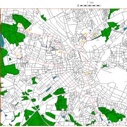
City of Osnabrück - traveling salesman (click to enlarge):

Further Links (related software, SQL reference etc).