
| GRASS 5.7: Examples from US National Atlas |
| Getting the data |
The data sets are available from the
National Atlas of the United States, in
particular from the Map Layers Warehouse
(this site is a dream for European GIS users).
We have to download following map layers:
LOCATION: nationalatlas mapset: user1 database: /usr/local/share/grassdata Please specify the coordinate system for locationB Latitude-Longitude Please enter a one line description for location > nationalatlas Do you wish to specify a geodetic datum for this location?(y/n) [y] y Please specify datum name >nad83 Now select Datum Transformation Parameters >6 # 6 Used in Default nad83 region DEFINE THE DEFAULT REGION ====== DEFAULT REGION ======= | NORTH EDGE:74:50N____ | | | WEST EDGE | |EAST EDGE 169:15E___ | |62:00W____ | SOUTH EDGE:13:20N____ | ============================= PROJECTION: 3 (Latitude-Longitude) ZONE: 0 GRID RESOLUTION East-West: 0:05______ North-South: 0:05______
The data sets are provided in SHAPE format as well as SDTS format. GRASS can read both: A) Import of "Cities and Towns" as SHAPE file:
v.in.ogr dsn=citiesx020.shp output=cities
v.db.connect -p cities
d.vect cities icon=basic/circle fcolor=red
v.in.ogr dsn=CITXCATD.DDF output=CITX
v.db.connect -p CITX
d.vect CITX icon=basic/circle fcolor=red
NOTE: Due to the map/tables size zooming before running a query with 'd.what.vect' is recommended.
We continue to work with the SHAPE files. Import of the "States" map:
v.in.ogr dsn=statesp020.shp output=states
d.vect map=states fcolor=255:255:220
v.in.ogr dsn=statesp020.shp output=roads
d.vect map=roads where="FEATURE='Limited Access Highway   Toll Road' or FEATURE='Limited Access Highway'" col=blue
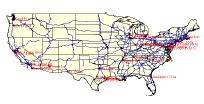
The maps imported so far look like this:

Ex 1) List the name and area of all the states that are adjacent to Minnesota in the State table.
d.what.vect states
#see attribute table

v.extract input=states output=minnesota where=STATE='Minnesota'
TODO - implement touch operator
Ex 3) List all the cities, which are within 150 km of the Interstate Route 90 road.
#we are using the STRING_MATCH operator '~':
d.vect map=roads where="NAME ~ 'Interstate Route 90'" col=green

v.extract input=roads output=interstate90 field=1 new=0 where="NAME ~ 'Interstate Route 90'"

# buffer is in map units, here geodetic dist in Lat/Long = some arc seconds:
v.buffer input=interstate90 output=interstate90_150km buffer=0:00:23 tolerance=1
TODO - implementation of cross operator
Further Links (related software, SQL reference etc).