Note: This document is for an older version of GRASS GIS that has been discontinued. You should upgrade, and read the current manual page.

NAME
r.random.surface - Generates random surface(s) with spatial dependence.KEYWORDS
raster, surface, randomSYNOPSIS
Flags:
- -u
- Uniformly distributed cell values
- --overwrite
- Allow output files to overwrite existing files
- --help
- Print usage summary
- --verbose
- Verbose module output
- --quiet
- Quiet module output
- --ui
- Force launching GUI dialog
Parameters:
- output=string[,string,...] [required]
- Name for output raster map(s)
- distance=float
- Maximum distance of spatial correlation (value >= 0.0)
- Default: 0.0
- exponent=float
- Distance decay exponent (value > 0.0)
- Default: 1.0
- flat=float
- Distance filter remains flat before beginning exponent
- Default: 0.0
- seed=integer
- Random seed, default [random]
- high=integer
- Maximum cell value of distribution
- Default: 255
Table of contents
DESCRIPTION
r.random.surface generates a spatially dependent random surface. The random surface is composed of values representing the deviation from the mean of the initial random values driving the algorithm. The initial random values are independent Gaussian random deviates with a mean of 0 and standard deviation of 1. The initial values are spread over each output map using filter(s) of diameter distance. The influence of each random value on nearby cells is determined by a distance decay function based on exponent. If multiple filters are passed over the output maps, each filter is given a weight based on the weight inputs. The resulting random surface can have any mean and variance, but the theoretical mean of an infinitely large map is 0.0 and a variance of 1.0. Description of the algorithm is in the NOTES section.The random surface generated are composed of floating point numbers, and saved in the category description files of the output map(s). Cell values are uniformly or normally distributed between 1 and high values inclusive (determined by whether the -u flag is used). The category names indicate the average floating point value and the range of floating point values that each cell value represents.
r.random.surface's original goal is to generate random fields for spatial error modeling. A procedure to use r.random.surface in spatial error modeling is given in the NOTES section.
Detailed parameter description
- output
- Random surface(s). The cell values are a random distribution between the low and high values inclusive. The category values of the output map(s) are in the form #.# #.# to #.# where each #.# is a floating point number. The first number is the average of the random values the cell value represents. The other two numbers are the range of random values for that cell value. The average mean value of generated output map(s) is 0. The average variance of map(s) generated is 1. The random values represent the standard deviation from the mean of that random surface.
- distance
- Distance determines the spatial dependence of the output map(s). The distance value indicates the minimum distance at which two map cells have no relationship to each other. A distance value of 0.0 indicates that there is no spatial dependence (i.e., adjacent cell values have no relationship to each other). As the distance value increases, adjacent cell values will have values closer to each other. But the range and distribution of cell values over the output map(s) will remain the same. Visually, the clumps of lower and higher values gets larger as distance increases. If multiple values are given, each output map will have multiple filters, one for each set of distance, exponent, and weight values.
- exponent
- Exponent determines the distance decay exponent for a particular filter. The exponent value(s) have the property of determining the texture of the random surface. Texture will decrease as the exponent value(s) get closer to 1.0. Normally, exponent will be 1.0 or less. If there are no exponent values given, each filter will be given an exponent value of 1.0. If there is at least one exponent value given, there must be one exponent value for each distance value.
- flat
- Flat determines the distance at which the filter.
- weight
- Weight determines the relative importance of each filter. For example, if there were two filters driving the algorithm and weight=1.0, 2.0 was given in the command line: The second filter would be twice as important as the first filter. If no weight values are given, each filter will be just as important as the other filters defining the random field. If weight values exist, there must be a weight value for each filter of the random field.
- high
- Specifies the high end of the range of cell values in the output map(s). Specifying a very large high value will minimize the errors caused by the random surface's discretization. The word errors is in quotes because errors in discretization are often going to cancel each other out and the spatial statistics are far more sensitive to the initial independent random deviates than any potential discretization errors.
- seed
- Specifies the random seed(s), one for each map, that r.random.surface will use to generate the initial set of random values that the resulting map is based on. If the random seed is not given, r.random.surface will get a seed from the process ID number.
NOTES
While most literature uses the term random field instead of random surface, this algorithm always generates a surface. Thus, its use of random surface.r.random.surface builds the random surface using a filter algorithm smoothing a map of independent random deviates. The size of the filter is determined by the largest distance of spatial dependence. The shape of the filter is determined by the distance decay exponent(s), and the various weights if different sets of spatial parameters are used. The map of independent random deviates will be as large as the current region PLUS the extent of the filter. This will eliminate edge effects caused by the reduction of degrees of freedom. The map of independent random deviates will ignore the current mask for the same reason.
One of the most important uses for r.random.surface is to determine how the error inherent in raster maps might effect the analyses done with those maps.
EXAMPLE
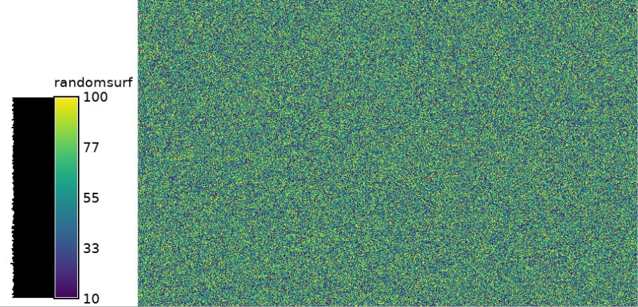
Generate a random surface (using extent of North Carolina sample dataset):g.region raster=elevation res=100 -p r.surf.random output=randomsurf min=10 max=100 # verify distribution r.univar -e map=randomsurf
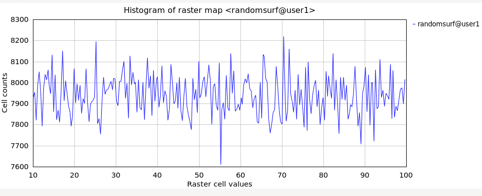
With the histogram tool the cell values versus count can be shown.
REFERENCES
Random Field Software for GRASS by Chuck EhlschlaegerAs part of my dissertation, I put together several programs that help GRASS (4.1 and beyond) develop uncertainty models of spatial data. I hope you find it useful and dependable. The following papers might clarify their use:
- Ehlschlaeger, C.R., Shortridge, A.M., Goodchild, M.F., 1997. Visualizing spatial data uncertainty using animation. Computers & Geosciences 23, 387-395. doi:10.1016/S0098-3004(97)00005-8
- Ehlschlaeger, C.R., Shortridge, A.M., 1996. Modeling Uncertainty in Elevation Data for Geographical Analysis. Proceedings of the 7th International Symposium on Spatial Data Handling, Delft, Netherlands, August 1996.
- Ehlschlaeger, C.R., Goodchild, M.F., 1994. Dealing with Uncertainty in Categorical Coverage Maps: Defining, Visualizing, and Managing Data Errors. Proceedings, Workshop on Geographic Information Systems at the Conference on Information and Knowledge Management, Gaithersburg MD, 1994.
- Ehlschlaeger, C.R., Goodchild, M.F., 1994. Uncertainty in Spatial Data: Defining, Visualizing, and Managing Data Errors. Proceedings, GIS/LIS'94, pp. 246-253, Phoenix AZ, 1994.
SEE ALSO
r.random, r.random.cells, r.mapcalc, r.surf.randomAUTHORS
Charles Ehlschlaeger, Michael Goodchild, and Chih-chang Lin; National Center for Geographic Information and Analysis, University of California, Santa BarbaraSOURCE CODE
Available at: r.random.surface source code (history)
Latest change: Sunday Feb 12 15:51:56 2023 in commit: 7d6ff54e985c1579e11b74c230cb8fa68a9aa928
Main index | Raster index | Topics index | Keywords index | Graphical index | Full index
© 2003-2024 GRASS Development Team, GRASS GIS 8.3.3dev Reference Manual

