NAME
v.lidar.mcc - Reclassifies points of a LiDAR point cloud as ground / non-ground using a multiscale curvature based classification algorithm.KEYWORDS
vector, lidar, classificationSYNOPSIS
Flags:
- -n
- Filter negative outliers (default is positive)
- --overwrite
- Allow output files to overwrite existing files
- --help
- Print usage summary
- --verbose
- Verbose module output
- --quiet
- Quiet module output
- --ui
- Force launching GUI dialog
Parameters:
- input=name [required]
- Input point layer
- Input vector point map
- ground=name [required]
- Output ground return points
- Output vector point map containing points classified as ground return
- nonground=name [required]
- Output non-ground return points
- Output vector point map containing points NOT classified as ground return
- nl=integer
- Number of scale domains (nl)
- nl
- Default: 3
- t=float
- Curvature tolerance threshold (t)
- Default: 0.3
- j=float
- Convergence threshold (j)
- Default: 0.1
- f=float
- Tension parameter (f)
- Default: 2
- s=integer
- Spline steps parameter (s)
- Default: 10
Table of contents
DESCRIPTION
v.lidar.mcc is a modified implementation of the Multiscale Curvature Classification (MCC) algorithm proposed by Evans & Hudak 2007.
The aim of the MCC-procedure is to filter non-ground returns caused by vegetation cover from point clouds
produced with any kind of LiDAR instrument (e.g. also instruments without intensity information).
The basic principle of the algorithm is to classify those points as non-ground points which deviate more than a user-defined threshold (t) from a surface which was interpolated from the full point cloud as a thin plate (here implemented with a bilinear spline interpolation with Tykhonov regularization through v.outlier). Tension (f) and spline steps (s) parameter are passed to the relevant parameters in v.outlier.
On each scale domain v.lidar.mcc calls v.outlier repeatedly until the algorithm converges, i.e. less than the amount of points (percentage of input points to the iteration) defined in the convergence threshold (j) are classified as non-ground points. Scale domains are defined in relation to the current region. With a number of scale domains (nl) greater than 1 scale domains are distributed evenly "around" the current region. With the default number of three scale domains, the first scale domaine uses half the resolution of the current region, scale domain two uses the current region and scale domain three uses 1,5 times the resolution of the current region.
NOTES
The optimal settings for the parameters of v.lidar.mcc depend very much on the resolution of the current region and the density of the LiDAR data, as well as terrain and vegetation. Therefore, a bit of try and error is usually required in order to find the optimal settings. In general spline steps (s) and curvature tolerance threshold (t) parameters have most influence on the results, where larger spline steps and a lower curvature tolerance threshold lead to more points clasified as non-ground points, but possibly also to increased clasification errors in complex terrain.
The algorithm by Evans & Hudak 2007 was developed for filtering LiDAR data in dense forest areas where not necessarily all pixels have a ground return point which is why a simple local minimum filering often is not sufficient.
In principle the algorithm works also on shrub-vegetation, however due to the lower vegetation type the curvature threshold will have to be lowered. In this case special attention should be payed to edges and peaks in the terrain which may be affected by low curvature tolerance thresholds. Therfore using a smaller cell size and wider spline steps is recommended for filtering lower structures like shrubs.
The effect and output of the filtering process can be visually inspected already during iterations when the resulting layer with non-ground points is
displayed while the classification is running.
However, especially the first runs on scale domains with a small pixels size can be relatively time consuming.
EXAMPLES
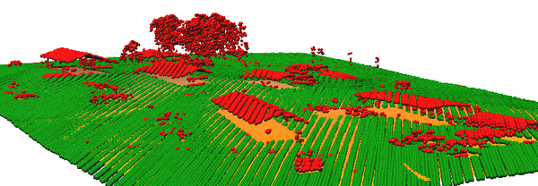
Classifying ground points in a LIDAR point cloud:# region settings (using an existing raster) g.region raster=elev_lid792_1m # import v.in.lidar -tr input=points.las output=points # classification v.lidar.mcc points ground=ground_points nonground=non_ground_points

Figure: Ground points (green) and non ground points (red)
SEE ALSO
v.surf.bspline, v.outlier, v.lidar.edgedetectionREFERENCES
Evans, J. S. & Hudak, A. T. 2007: A Multiscale Curvature Algorithm for Classifying Discrete Return LiDAR in Forested Environments. IEEE TRANSACTIONS ON GEOSCIENCE AND REMOTE SENSING 45(4): 1029 - 1038. https://www.fs.usda.gov/rm/pubs_other/rmrs_2007_evans_j001.pdfhttps://sourceforge.net/p/mcclidar/wiki/Home/
AUTHOR
Stefan Blumentrath, Norwegian Institute for Nature Research (NINA), Oslo, NorwaySOURCE CODE
Available at: v.lidar.mcc source code (history)
Latest change: Tuesday Feb 17 14:54:26 2026 in commit: 051b9c19442e746e2b51f9c5382809a45230b4c0
Main index | Vector index | Topics index | Keywords index | Graphical index | Full index
© 2003-2025 GRASS Development Team, GRASS GIS 8.4.3dev Reference Manual