Jupyter notebooks introduction
The grass.jupyter Python package provides a Jupyter
notebook interface to GRASS. It includes modules for creating map figures,
interactive web maps, visualizing data series and time series, and generating
3D visualizations.
If you don't have a project yet, create a new one first:
import grass.script as gs

gs.create_project("path/to/my_project", epsg="3358")
To get started with grass.jupyter, import the package,
and start a GRASS session with the gj.init function:
import grass.jupyter as gj

session = gj.init("path/to/my_project")
Now you can import raster or vector data with r.import and v.import. The following examples will use the North Carolina dataset.
Importing packages
To import the grass.script and grass.jupyter packages, you need to tell Python where the GRASS Python package is unless you are running a notebook in a GRASS session.
import sys
import subprocess

sys.path.append(
    subprocess.check_output(["grass", "--config", "python_path"], text=True).strip()
)
Mapsets
If not specified otherwise in the gj.init function, the session will
start in the default
mapset (subproject) of a project. If you need later to switch to a
different mapset, you can use the gj.switch_mapset function.
Map
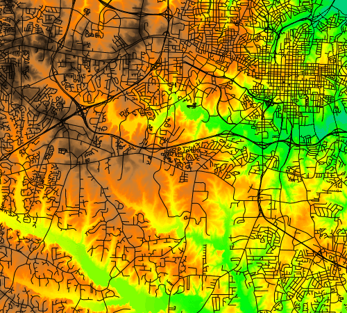
The gj.Map class in grass.jupyter provides a way to create static maps in Jupyter.
Here we create a map of elevation overlayed with streets:
# Create a new map
m = gj.Map()

# Add a raster map to the map object
m.d_rast(map="elevation")

# Add a vector map to the map object
m.d_vect(map="streets", color="black")

# Display the map
m.show()
Order Matters
Map features are added to the map in the order they are called. For example, if you add a raster map and then a vector map, the vector map will be drawn on top of the raster map.
In addition to displaying raster and vector maps, the gj.Map can access many
of the display tools in GRASS. For a complete list of cartographic
features you can refer to the Cartography topic page.
For example, let's add a legend, barscale, and shaded relief to the map:
from grass.tools import Tools

# Create an object to access tools
tools = Tools()

# Compute shaded relief
tools.r_relief(input="elevation", output="relief")

# Create a new map
m = gj.Map()

# Add a shaded relief map
m.d_shade(color="elevation", shade="relief")

# Add a raster legend
m.d_legend(
    raster="elevation",
    at=(1, 50, 1, 8),
    title="Elevation (m)",
    border_color="none",
    flags="bt"
)

# Add a scale bar to the map
m.d_barscale(at=(55, 5), flags="n")

# Display the map
m.show()
Map Size and Extent
See detailed documentation for changing the map size and geographic extent.
Interactive map
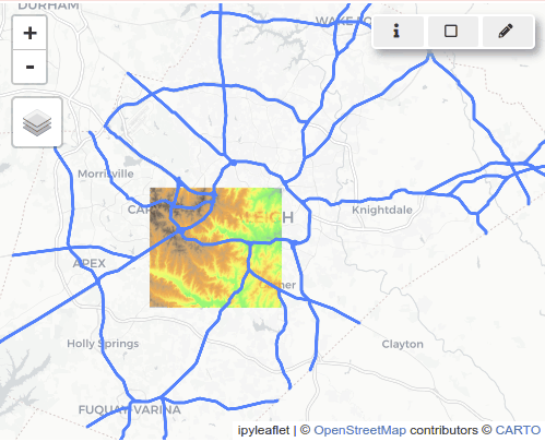
The gj.InteractiveMap class provides a way to create interactive
web maps in Jupyter. Interactive maps are created using the
ipyleaflet
or folium libraries.
The default is ipyleaflet,
which gives you more interactivity and control over the map. Here we create
an interactive map of the elevation raster and the roadsmajor
vector map:
# Create an interactive map
m = gj.InteractiveMap()
m.add_raster("elevation", opacity=0.7)
m.add_vector("roadsmajor")
m.show()
The map gives you the ability to query the map, zoom in and out, and pan around, set the computational region, and create simple vector data by digitizing. To change the default basemap, see documentation.
3D map
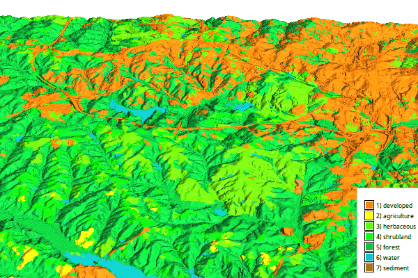
The gj.Map3D class creates 3D visualizations as static images.
elevation_3dmap = gj.Map3D()
elevation_3dmap.render(
    elevation_map="elevation",
    color_map="landuse",
    position=[0.5, 1],
    perspective=10,
    height=5000,
    resolution_fine=1,
    zexag=5
)
elevation_3dmap.overlay.d_legend(raster="landuse",
                                 at=(0, 30, 87, 100),
                                 flags="b",
                                 border_color="none")
elevation_3dmap.show()
The parameters of the render() function are the same as parameters of the
m.nviz.image tool, which is used in the background.
Series map
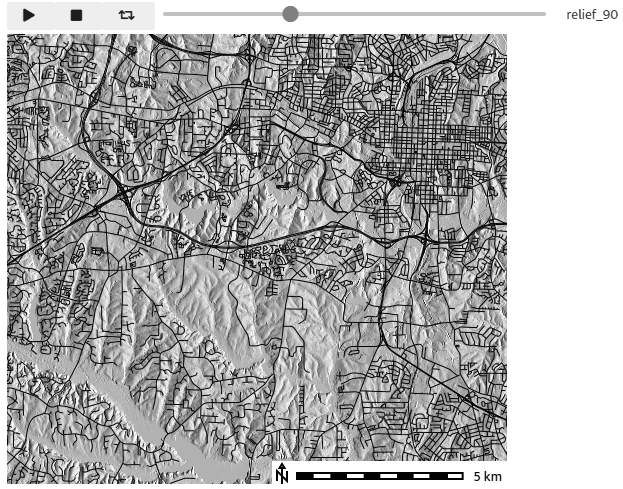
The gj.SeriesMap class animates a series of maps, allowing users to slide between
maps and play a continuous loop.
# Create a series of relief maps with different angles
directions = [0, 90, 180, 270]
for azimuth in directions:
    tools.r_relief(
        input="elevation",
        output=f"relief_{azimuth}",
        azimuth=azimuth)
m = gj.SeriesMap()
m.add_rasters(f"relief_{azimuth}" for azimuth in directions)
m.d_vect(map="roads")
m.d_barscale(at=(80, 10))
m.show()
# Save the map as animated gif
m.save("series_map.gif")
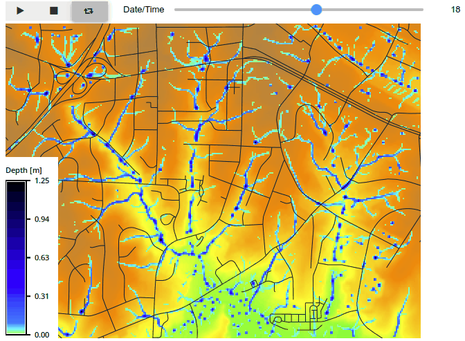
Time series map
The gj.TimeSeriesMap class provides a way to visualize
GRASS' space time datasets in Jupyter. Here we create a time
series map of overland water flow:
# Zoom in to the study area
tools.g_region(n=226040, s=223780, e=639170, w=636190)
# Compute topography dx and dy derivatives
tools.r_slope_aspect(elevation="elevation", dx="dx", dy="dy")
# Compute overland flow
tools.r_sim_water(
    flags="t",
    elevation="elevation",
    dx="dx",
    dy="dy",
    depth="depth",
    duration=30)

# Create a time series
tools.t_create(
    output="depth",
    temporaltype="relative",
    title="Overland flow depth",
    description="Overland flow depth")
# Register the time series
maps = [
    item["fullname"]
    for item in tools.g_list(type="raster", pattern="depth*", format="json")
]
tools.t_register(input="depth", maps=maps)

# Create a time series map
flow_map = gj.TimeSeriesMap()

# Add the base map
flow_map.d_rast(map="elevation")
# Add the time series data
flow_map.add_raster_series("depth", values="0.025-1.25")
# Overlay the vector map
flow_map.d_vect(map="streets")

# Add map features
flow_map.d_legend(raster="depth.30",
                  title="Depth [m]",
                  flags="bt",
                  border_color="none",
                  at=(1, 50, 0, 5))

# Display the map
flow_map.show()
Python library documentation
For complete documentation on the grass.jupyter package, see the
grass.jupyter
library documentation page.
For complete documentation on the grass.tools package, see the
grass.tools
library documentation page.
For complete documentation on the grass.script package, see the
grass.script
library documentation page.
Tutorials
- Get started with GRASS in Jupyter Notebooks on Windows
- Get started with GRASS & Python in Jupyter Notebooks (Unix/Linux)
- Get started with GRASS in Google Colab
- Run
grass.jupytertutorial on Binder:
SOURCE CODE
Available at: jupyter_intro source code
(history)
Latest change: Thursday Mar 12 19:34:43 2026 in commit 4334ea5
